
Algorithms
All downloadable material listed on these pages - appended by specifics mentioned under the individual headers/chapters - is available for public use. Please note that while great care has been taken, the software, code and data are provided "as is" and that Food Analytics and Biotechnology at UCPH does not accept any responsibility or liability.
Tools for hyperspectral analysis --> New version with GUI available the 1st of August
THE NEW HYPER-Tools is available here:
Variable selection in high dimensional models can improve the interpretability and performance. One way to achieve sparsity is through penalized minimization problems with bounding of the $L_1$ norm of some parameter entity. This concept has received huge attention within fields such as statistical learning, data mining, signal processing.
SPARAFAC (Sparse PARAFAC)
In sparse principal component analysis the aim is to estimate a PARAFAC-like model where sparsity is induced on the model parameters. Sparsity in several modes is (here) referred to as multidimensional co-clustering.
Download algorithm
An algorithm for estimation of a SPARAFAC model can be downloaded here.
References:
Rasmussen MA and Bro R (2012) A tutorial on the LASSO approach to sparse modelling, Chemometrics and Intelligent Laboratory Systems, 119,21:31
Algorithmic details
Solving a constrained optimization problems like:
Input: $\mathbf{X}$ - data, $k$ - number of components, $\lambda$ - penalty from the Lagrangian formulation, additional constraints (nonnegativity and orthogonality (not defined for otherwise constrained components))
Initialize with random numbers, tucker3 solution or unconstrained PARAFAC.
For i=1,...,
- Estimate $\mathbf{A}$ when $\mathbf{B}$ and $\mathbf{C}$ is fixed.
- Estimate $\mathbf{B}$ when $\mathbf{A}$ and $\mathbf{C}$ is fixed.
- Estimate $\mathbf{C}$ when $\mathbf{A}$ and $\mathbf{B}$ is fixed.
Repeat 1-3 until convergence
Due to similarities with the Alternating Least Squares (ALS) algorithm, a name could be Alternating Shrunken Least Squares (ASLS).
As none of these problems are convex, a solution might be a local minimum. Hence multible starts for determing local solutions are needed.
Soft thresholding
Estimation of $\mathbf{p}$ when $\mathbf{t}$ is known correspond to solving: $ \mathrm{min}(\frac{1}{2}\left|\mathbf{X} - \mathbf{t}\mathbf{p}^T\right|_F^2 + \lambda\left|\mathbf{p}\right|_1) $ with respect to $\mathbf{p}$. Seeting $\mathbf{p_{LS}} = (\mathbf{t}^T\mathbf{t})^{-1}\mathbf{t}^T\mathbf{X} $ to the least squares solution, the solution is a soft thresholded version of $\mathbf{p_{LS}}$ by $\lambda$:
$$ p_j = S(p_{LSj},\lambda) $$
Below is exemplified how this operator works.

drEEM - Matlab toolbox supporting visualisation and PARAFAC of excitation emission matrices (EEMs)drEEM - Matlab toolbox supporting visualisation and PARAFAC of excitation emission matrices (EEMs)drEEM - Matlab toolbox supporting visualisation and PARAFAC of excitation emission matrices (EEMs)drEEM - Matlab toolbox supporting visualisation and PARAFAC of excitation emission matrices (EEMs)
Some fields where calibration of multi-way data is required, such as hyphenated chromatography, can suffer of high inaccuracy when traditional N-PLS is used, due to the presence of shifts or peak shape changes in one of the modes. To overcome this problem, a new regression method for multi-way data called SCREAM (Shifted Covariates REgression Analysis for Multi-way data), which is based on a combination of PARAFAC2 and principal covariates regression (PCovR), is proposed. In particular, the algorithm combines a PARAFAC2 decomposition of the X array and a PCovR-like way of computing the regression coefficients, analogously to what has been described by Smilde and Kiers (A.K. Smilde and H.A.L. Kiers, 1999) in the case of other multi-way PCovR models. The method is tested on real and simulated datasets providing good results and performing as well or better than other available regression approaches for multi-way data.
Reference:
If you use SCREAM, we would appreciate a link to
F. Marini and R. Bro. SCREAM: A novel method for multi-way regression problems with shifts and shape changes in one mode. Chemom.Intell.Lab.Syst. 129:64-75, 2013.
Sparsity
Variable selection in high dimensional models can improve the interpretability and performance. One way to achieve sparsity is through penalized minimization problems with bounding of the $L_1$ norm of some parameter entity. This concept has received huge attention within fields such as statistical learning, data mining, signal processing.
PCA (Sparse PCA)
In sparse principal component analysis the aim is to estimate a PCA-like model where sparsity is induced on the model parameters; scores or loadings. Sparsity in both modes is (here) referred to as co-clustering.
SPCA, with sparsity constraint on loadings, can be formulated as:
$$ \mathrm{min}(\left|\mathbf{X} - \mathbf{T}\mathbf{P}^T\right|_F^2) $$
subject to
$$ \left|\mathbf{p}_i\right|_1 \leq c, for \ i=1,...,k $$
where $\mathbf{X} (n \times p) $ is the data matrix, $\mathbf{T} (n \times k) $ is the score matrix and $\mathbf{P} = [\mathbf{p_1} \ldots \mathbf{p_k}]$ $(p \times k)$ is the loading matrix. $k$ is the number of components.$\left|\cdot\right|_F$ is the Frobenius norm (sum of the squared elements).
This can, for each component, be formulated as a single object function (Lagrangian):
$$ \mathrm{min}(\left|\mathbf{X} - \mathbf{t}\mathbf{p}^T\right|_F^2 + \lambda\left|\mathbf{p}\right|_1) $$
Choosing an appropriate value for $\lambda$ (or $c$) leads to a sparse solution, i.e. several of the loadings are exactly zero.
OBS: There is not an easy translation from $c$ to $\lambda$, and for estimation of more than one component, one has to choose whether to fix $c$ or $\lambda$.
Download algorithm
An algorithm for estimation of a SPCA model can be downloaded here. Details are described in the section Algorithms below.
Example
12 samples of jam corresponding to a full factorial design of four locations and three harvest times are evaluated on six instrumental parameters and 13 sensory attributes. Data can be downloaded here.
In the figure below results from PCA (stems) and SPCA (bars) are compared.
 and SPCA (bars)")
SPCA/PCA figure Score plot (A and B) with color reflecting harvest time (component 1) and location (component 2). Loading plot (C and D).
Interpreting the loadings (C and C) reveals that the SPCA deselects some of the low influencing variables, and thereby leading to more interpretable components.
References:
Rasmussen MA and Bro R (2012) A tutorial on the LASSO approach to sparse modelling, Chemometrics and Intelligent Laboratory Systems, 119,21:31
Shen, H. and Huang, J.Z. (2008) Sparse principal component analysis via regularized low rank matrix approximation, Journal of multivariate analysis, 99,6:1015-1034
Algorithmic details
Solving a constrained optimization problems like:
$$ \mathrm{min}(\left|\mathbf{X} - \mathbf{T}\mathbf{P}^T\right|_F^2) s.t. \left|\mathbf{p}_i\right|_1 \leq c, for \ i=1,...,k $$
Is a nested convex problem. This means that for fixed loadings ($\mathbf{P}$), calculating the scores ($\mathbf{T}$) is a convex problem. Estimation of loadings with fixed scores ($\mathbf{T}$) is a componentwise convex problem. This advocates for an iterative alternating procedure. In case of nested components the procedure looks something like this.
Input: $\mathbf{X}$ - data, $k$ - number of components, $\lambda$ - penalty from the Lagrangian formulation.
For j=1:k
Initialize with ordinary $1$ component PCA solution $\mathbf{X} = \mathbf{t}\mathbf{p}^T$
For i=1,...,
- Estimate $\mathbf{t}$ when $\mathbf{p}$ is known: $\mathbf{t} = \mathbf{X}\mathbf{p}$
- Estimate $\mathbf{p}$ when $\mathbf{t}$ is known: By soft thresholding
Repeat 1-2 until convergence
Deflate: $\mathbf{X} = \mathbf{X} - \mathbf{t}\mathbf{p}^T$
Repeat up to k components
Due to similarities with the Non linear Iterative PArtial Least Squares (NIPALS) algorithm, and the fact that softthresholding works on the least squares estimates, a name could be Non linear Iterative PAtial Shrunken Least Squares (NIPASLS).
Calculation of components based on the current residuals, do not directly aim at solving $ \mathrm{min}(\left|\mathbf{X} - \mathbf{T}\mathbf{P}^T\right|_F^2) s.t. \left|\mathbf{p}_i\right|_1 \leq c, for \ i=1,...,k $, as the components in spca are not orthogonal. A more direct approach where the entire set of components are estimated simultaneously by iterating between scores and loadings can hence be considered. This goes as follows:
Input: $\mathbf{X}$ - data, $k$ - number of components, $\lambda$ - penalty from the Lagrangian formulation.
Initialize with ordinary $k$ component PCA solution
For i=1,...,
- Estimate $\mathbf{T}$ when $\mathbf{P}$ is known: $\mathbf{T} = \mathbf{X}\mathbf{P}^+$
- Estimate $\mathbf{P}$ when $\mathbf{T}$ is known: By componentwise soft thresholding of least squares estimates.
Repeat 1-2 until convergence
$\mathbf{P}^+$ is the pseudo inverse of $\mathbf{P}$
Due to similarities with the Alternating Least Squares (ALS) algorithm, a name could be Alternating Shrunken Least Squares (ASLS).
As none of these problems are convex, a solution might be a local minimum. In the algorithm spca.m for Matlab both options (ASLS and NIPASLS) are available
Soft thresholding
Estimation of $\mathbf{p}$ when $\mathbf{t}$ is known correspond to solving: $ \mathrm{min}(\frac{1}{2}\left|\mathbf{X} - \mathbf{t}\mathbf{p}^T\right|_F^2 + \lambda\left|\mathbf{p}\right|_1) $ with respect to $\mathbf{p}$. Seeting $\mathbf{p_{LS}} = (\mathbf{t}^T\mathbf{t})^{-1}\mathbf{t}^T\mathbf{X} $ to the least squares solution, the solution is a soft thresholded version of $\mathbf{p_{LS}}$ by $\lambda$:
$$ p_j = S(p_{LSj},\lambda) $$
Below is exemplified how this operator works.

Dietary Patterns
Dietary patterns better reflect eating habits as opposed to single dietary components. However, the use of dietary pattern analysis in nutritional epidemiology has been hampered by the complexity of interpreting and presenting multidimensional dietary data.
Analysis of dietary data
Dietary data often consists of registrations of a range of different food items or products such as tomatoes, beans, low fat milk etc. with a total of 30 to 80 food items. The aim of dietary pattern analysis is to extract certain patterns which constitute certain eating habits. This is most often done with no a priory information and solely based on the relational (correlation) structure within in the data. A natural choice is to use principal component analysis (PCA - for a detailed description click here), possibly with a simplicity-rotation, for estimation of patterns. The outcome form a PCA analysis is two sets of related sources of information, often referred to as factor scores and factor loadings. The factor loadings constitute the structure of the factor with respect to the food items and hence reflect which food items that are 1) responsible for the factor and 2) how these are correlated. The factor scores constitute a measure of how much the individual person has of this certain component.
Factor scores
The factor scores can be used as a measure of intake in the same way as the original data, and hence be used for comparison with socio demographic information or certain health related outcomes. The only difference between the factor score for say western diet and the food item say low-fat milk is that the scale of the factor score is arbitrary.
Factor loadings

The factor loading carry the information on the signature of dietary pattern and is therefor central in the translation of the factor into something meaningful. It and naming is the factor loadings that give rise to naming of the factor and to interpretation of an association between the factor score and certain outcomes. It is therefor of utmost importance, that the factor loadings are presented as clear as possible. Tabulation of factor loadings for more than 30 variables demands exhaustive reading in order to capture all details. Visualization of factor loadings, does however, guide the eye towards what is important.
Visualization tools
Spiderplot - TO APPEAR
In this interface you can provide an .xls(x) file with information on the factor structure (names of food items, partition into groups of food items and factor correlation) which then will make a spiderplot. Download the following file and modify to fit your own results.
Backbone matlab files
The file spideplot.m can be used for the same purpose as the interface for those who have matlab locally on their machine.
References
Hu FB (2002) Dietary pattern analysis: a new direction in nutritional epidemiology, Current Opinion in Lipidology, 13:3–9
Rasmussen MA, Maslova E, Halldorsson TI, Olsen SF, Characterization of Dietary Patterns in the Danish National Birth Cohort in relation to preterm birth. submitted to American journal of epidemiology
”Recursive weighted partial least squares" (rPLS)

Variable selection is important in fine tuning partial least squares (PLS) regression models. This method is a novel variable weighting method for PLS regression where the univariate response variable y is used to guide the variable weighting in a recursive manner — the method is called recursive weighted PLS or just rPLS. The method iteratively reweights the variables using the regression coefficients calculated by PLS. The use of the regression vector to make up the weights is a reasonable idea from the fact that the weights in the regression vector ideally reflect the importance of the variables. In contrast to many other variable selection methods, the rPLS method has the advantage that only one parameter needs to be estimated: the number of latent factors used in the PLS model. The rPLS model has the fascinating output that it, under normal conditions, converges to a very limited number of variables (useful for interpretation), but it will exhibit optimal regression performance before convergence, normally including covarying neighbour variables.
Reference / If you use rPLS, we would appreciate a link to:
Å. Rinnan, M. Andersson, C. Ridder and S. B. Engelsen: Recursive weighted partial least squares (rPLS): an efficient variable selection method using PLS, Journal of Chemometrics, DOI: 10.1002/cem.2582.
Version 1.0
The function AutoChrome is an expert system that can find the number of PARAFAC2 components needed for modeling a given (narrow) set of peaks.
Reference:
If you use AutoChrome we would appreciate a citation to:
Johnsen, Amigo, Skov, Bro, Automated resolution of overlapping peaks in chromatographic data, Journal of Chemometrics, DOI: 10.1002/cem.2575
Downloads:
AutoChrome version 1
Note that AutoChrome requires PLS_Toolbox to function
by Mikkel Brydegaard, Lund Laser Centre, Lund University, Sweden, Mikkel.brydegaard@fysik.lth.se
and Yoel Stuart, Department of Organismic and Evolutionary Biology, Harvard University, Cambridge, Massachusetts, USA
(v1.0, Sep. 2013)
")
Introduction
This tutorial and software package demonstrates the concept of multidimensional chromatic distribution and examples on how to use such. Multi-dimensional chromatic distributions can be produces from widely available RGB color imagers, and is a straightforward way to capture arbitrary chromatic distributions and compare them in-between samples. The concept can be expanded to cover multispectral images [1]. The figure below illustrates why variance matters and one example where spatial chromatic variance is needed to identify the species. More considerations can be found in the authors reference [2] and in the included power point presentation.
Full toolbox (180MB, including source code, documentation, examples, etc.) find the toolbox needed from the list.
[1] S. Kucheryavskiy, "A new approach for discrimination of objects on hyperspectral images," Chemometrics and Intelligent Laboratory Systems, vol. 120, pp. 126-135, 2013.
[2] M. Brydegaard, A. Runemark, and R. Bro, "Chemometric approach to chromatic spatial variance. Case study: patchiness of the Skyros wall lizard," J. Chemometrics, pp. n/a-n/a, 2012.
POLYS 2.0
An open source software package for building three dimensional structures of polysaccharides

POLYS 2.0 DOWNLOAD
From the bitbucket repositoire (always latest version):
hg clone (includes source): https://bitbucket.org/polys/polys (doesn't work anymore)
or alternatively by direct download:
Installation on Linux/UNIX:
1. Go the the source code directory
2. Type 'make all'
3. Setup your shell environment as described in the INSTALL file.
Installation on Windows:
Bootstrap based Confidence Limits in Principal Component Analysis
The following code is a free MATLAB function to construct non-parametric bootstrap Bias-corrected and accelerated (BCa) confidence limits in PCA for scores and loadings. Further outputs are provided, e.g., bootstrap estimates of scores and loadings, standard error, and bias. Bootstrap confidence limits are useful to evaluate the uncertainty associated with samples or variables for outlier detection and variable selection.
In an experiment, NIR spectra of 2-Propanol/water mixtures were collected at two temperatures (data included in the download below):

The data were used to build non-parametric bootstrap BCa confidence intervals for PCA scores and loadings, where a PCA model with one PC was fitted to the bootstrap samples. The loading CIs are larger for the some variables compared to the others. The explanation is that the difference in the signal of the two sets is larger for those variables:

Please refer to the below paper when using the function:
H. Babamoradi, F. van den Berg, Å. Rinnan, Bootstrap based confidence limits in principal component analysis — A case study, Chemometrics Intellig. Lab. Syst. 120(2013)97-105
Download: PCA bootstrap (May 31st, 2013)
The MATLAB CMTF Toolbox has two different versions of the Coupled Matrix and Tensor Factorization (CMTF) approach used to jointly analyze datasets of different orders: (i) CMTF and (ii) ACMTF. First-order unconstrained optimization is used to fit both versions. The MATLAB CMTF Toolbox has the functions necessary to compute function values and gradients for CMTF and ACMTF. For the optimization routines, it uses the Poblano Toolbox. The Tensor Toolbox is also needed to run the functions in the MATLAB CMTF Toolbox.
In order to learn about the coupled models in the toolbox and see example scripts showing how to use CMTF and ACMTF, please visit the examples for toolboxes and code.
What is new in Version 1.1? (Dec., 2014)
- Compatibility with sptensor is added to make CMTF_OPT and ACMTF_OPT work with tensors in sptensor form.
- TESTER_CMTF and TESTER_ACMTF have been modified to have the option of generating data sets in dense or sparse tensor format.
- TESTER_CMTF_MISSING and TESTER_ACMTF_MISSING functions have been added to demonstrate the use of CMTF_OPT and ACMTF_OPT with data sets with missing entries.
- CREATE_COUPLED_SPARSE function has been added to generate coupled sparse data sets using sparse factor matrices.
- For smooth approximation of the l1-terms in SCP_FG, SCP_WFG, SPCA_FG, SPCA_WFG, eps is set to 1e-8.
Download the latest version: The MATLAB CMTF Toolbox (v1.1) (released Dec., 2014)
Older versions: The MATLAB CMTF Toolbox (v1.0) (released April, 2013)
References: If you use the MATLAB CMTF Toolbox, please cite the software along with the relevant publication:
- Article on CMTF: E. Acar, T. G. Kolda, and D. M. Dunlavy, All-at-once Optimization for Coupled Matrix and Tensor Factorizations, KDD Workshop on Mining and Learning with Graphs, 2011 (arXiv:1105.3422v1)
- Articles on ACMTF:
- E. Acar, A. J. Lawaetz, M. A. Rasmussen, and R. Bro, Structure-Revealing Data Fusion Model with Applications in Metabolomics,Proceedings of 35th Annual International Conference of the IEEE Engineering in Medicine and Biology Society (IEEE EMBC'13), pp. 6023-6026, 2013.
- E. Acar, E. E. Papalexakis, G. Gurdeniz, M. A. Rasmussen, A. J. Lawaetz, M. Nilsson, R. Bro, Structure-Revealing Data Fusion, BMC Bioinformatics, 15: 239, 2014.
NSIMCA Toolbox: short User Guide
The essential structure of NSIMCA toolbox is described here as well as a few essential Guidelines. NSIMCA is written in MATLAB and requires Nway Toolbox 3.1, misstoolbox and a few basic statistics routine (all is included in the NSIMCA folder). The toolbox is available from Chemometrics Research (ucphchemometrics.com)
If you use the NSIMCA toolbox for MATLAB we would appreciate a reference to:
C. Durante, R. Bro, M. Cocchi, A classification tool for N-way array based on SIMCA methodology, Chemometrics & Intelligent Laboratory Systems. 106 (2011), 73-85.
If you have any questions, suggestions or comments please feel free to mail us (Marina Cocchi).
The NSIMCA toolbox consists of six main routines:
- NSIMCA.m (main computing models for each category)
- Nclass.m (classification routine making class assignment)
- toplot.m (routine calculating and making plots of SENS, SPEC, efficiency vs. number of factors. Asking user for best combination and saving SENS/SPEC tables for best)
- NSIMCA_QTplots.m (graphical routine to make “alternative SIMCA” T2 vs. Q plots for each class)
- make_Coomans_simca.m (routine to calculate and save distances to classes as in “original-SIMCA” and parameters for F-test)
- toplot_coomans.m (graphical routine to make Coomans plots)
Download: NSIMCA toolbox version 1.0
FastChrom – Processing of chromatographic data

FastChrom is a complete Matlab-based method for baseline correction, peak detection, and assignment (grouping) of similar peaks across samples. The method is especially useful for single-channel data (e.g. GC-FID), but can also be applied on multi-channel data (e.g. total ion chromatogram from GC-MS).
The newly developed method for baseline correction uses parts of the chromatographic signal as baseline; therefore less noise is present in the baseline corrected signal compared to just subtracting a globally fitted polynomial. The incorporated peak detection method incorporated detects all peaks present in the chromatograms which fulfil the requirements set by the user, and there is no need for recalibration if shifts occur.
In FastChrom peaks are grouped according to a maximal shift which can be set by the user. In the grouping step information about the density of peaks across samples are used in the positioning of the centre of the grouping windows.
In addition FastChrom offers the possibility of applying a retention time index to the identified peak groups. The index will be unaffected by shifts in retention time. This possibility eases identification and comparison between different experiments.
FastChrom is implemented in a graphical user interface and can therefore be used by people without programming skills.
For import of cdf files, iCDF is used (Skov T and Bro R.(2008) Solving fundamental problems in chromatographic analysis Analytical and Bioanalytical Chemistry, 390 (1): 281-285. LINK
DOWNLOAD FastChrom ver 1.1
If you use the software in your research please make a reference to the following manuscript:
Lea G. Johnsen, Thomas Skov, Ulf Houlberg and Rasmus Bro "An automated method for baseline correction, peak finding and peak grouping in chromatographic data", Submitted (2012)
Loads2Chrom – identify modelled peaks from GC-MS datasets

About Loads2Chrom
Chemometric models (e.g. PARAFAC, PARAFAC2, MCR) can help to separate and purify overlapping peaks in GC-MS datasets into unique elution time and mass spectral profiles. However, software incompatibilities have prevented the modeled mass spectra from being easily compared to mass spectral databases. Recently, new software was developed to allow the identification of modeled peaks via the open-source chromatography and mass spectrometry software OpenChrom. On this page you can download software to convert model loadings of GC-MS peaks to *.mpl files, used by OpenChrom. In OpenChrom, the loadings can be converted to other formats or identified using NIST11 and NIST08.
Directions for identifying model loadings using OpenChrom are in:
Murphy, K. R.; Wenig, P.; Parcsi, G.; Skov, T.; Stuetz, R. M., Characterizing odorous emissions using new software for identifying peaks in chemometric models of gas chromatography–mass spectrometry datasets. Chemom. Intell. Lab. 2012, 118:41-50
To match modelled GC-MS peaks with spectra in NIST databases via OpenChrom, you will need:
· One or more models (e.g. PARAFAC, PARAFAC2, MCR) of GC-MS peaks
· OpenChrom the open source chromatography software. Get it here.
· Either loads2chrom.m (runs with a licenced version of MATLAB) or loads2chrom_XX.zip (runs with the free MATLAB Compiler Runtime). This converts the model loadings from matrix format to the mpl format.
· Access to a NIST mass spectral database
Download Loads2Chrom
This download contains:
1. Loads2Chrom.m – MATLAB m-file that performs the conversion from matrix loadings to mpl format. Loadings are in data structures created in MATLAB or in the PLS_Toolbox for MATLAB.
2. Loads2Chrom_86.zip - Stand-alone executable for 32-bit (x86) Windows operating systems. Double-click on the icon to convert loadings in the OpenChromData folder from text files to mpl. Requires MATLAB Compiler Runtime 7.17 (MCR_R2012a_win32).
3. Loads2Chrom_64.zip - Stand-alone executable for 64-bit Windows operating systems. Double-click on the icon to convert loadings in the OpenChromData folder from text files to mpl. Requires MATLAB Compiler Runtime 7.17 (MCR_R2012a_win64).
4. netCDFload.m - MATLAB m-file that loads netCDF files from different chromatographic software packages, and exports them as 2-D matrices. Requires MATLAB R2011a or later. With earlier MATLAB versions, use iCDF (link doesn't work anymore).
Related links:
ChromTools web site (to come)
The Odour Laboratory at the University of New South Wales, Sydney
OpenChrom web site
NIST mass spectral databases
The FDOMcorr toolbox for MATLAB
Sept. 19, 2011
The FDOMcorr toolbox has been developed to simplify and automate the correction of dissolved organic matter (DOM) fluorescence (EEM) datasets and facilitate comparisons between datasets collected by different researchers.
The FDOMcorr toolbox version 1.6 consists of five MATLAB executable files (M-files) designed to run with a template:
- ReadInEEMs.m : loads individual EEMs into a 3D matrix in preparation for further processing.
- ReadInScans.m : loads individual scans into a 2D matrix in preparation for further processing.
- MatchSamples.m : inflates a smaller dataset X2 (e.g. blanks) to pair with samples in dataset X1 (e.g. sample EEMs).
- RamanIntegrationRange.m : calculates the optimal range of emission intensities for determining Raman areas from spectral datasets.
- FDOMcorrect.m : implements algorithms for correcting spectral data for instrument bias and calibrating intensities to standardized units.
- FDOMcorrect template.m : a template illustrating the steps for implementing the complete EEM correction process. The template should be adapted by the user to accommodate their datasets.
This toolbox version has been tested in MATLAB 2010a. While FDOMcorr ver. 1.6 includes revisions to increase its compatibility with earlier versions of MATLAB, it is possible that some early versions may not be able to execute all files.
References:
1. Murphy, K. R.; Butler, K. D.; Spencer, R. G. M.; Stedmon, C. A.; Boehme, J. R.; Aiken, G. R., (2010). The measurement of dissolved organic matter fluorescence in aquatic environments: An interlaboratory comparison. Environmental Science and Technology, 44, 9405–9412. Free download
2. Murphy, K. R. (2011), A note on determining the extent of the water Raman peak in fluorescence spectroscopy. Applied Spectroscopy. 65(2), 233-236
Links:
FDOMcorr:
Chemometrics Research (ucphchemometrics.com)
Trouble shooting and FAQ:
link virker ikke længere, besøg Chemometrics Research (ucphchemometrics.com) for mere info
SMR - Sparse matrix regression for co-clustering
Co-clustering is the tool of choice when only a smaller subset of variables are related to a specific grouping among some subjects. Hence, co-clustering allows a select number of objects to have particular behavior on a select number of variables.

This SMR algorithm is a beta version which will allow you to build a co-clustering just by selecting the number of co-clusters. Be aware that co-clustering is intrinsically difficult so problems with local minima may occur. Also be aware that the current algorithm works best with data that is fairly square and fairly discrete.
Other algorithms and code can be downloaded here
If you use the functions provided here, you may want to reference
- E. E. Papalexakis, N. D. Sidiropoulos, and M. N. Garofalakis. Reviewer Profiling Using Sparse Matrix Regression. 1214-1219. 2010. 2010 IEEE International Conference on Data Mining Workshops.
- E. E. Papalexakis and N. D. Sidiropoulos. Co-clustering as multilinear decomposition with sparse latent factors. 2011. Prague, Czech Republic. 2011 IEEE International Conference on Acoustics, Speech and Signal Processing.
- R. Bro, E. Acar, V. Papalexakis, N. D. Sidiropoulos, Coclustering, Journal of Chemometrics, 2012, 26, 256-263.
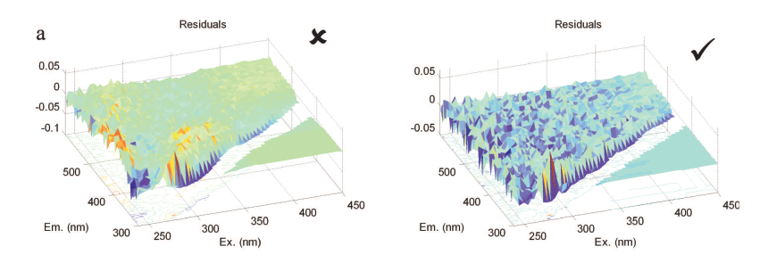
EEMizer: Automated modeling of fluorescence EEM data
PARAFAC offers a very attractive approach for modeling fluorescence excitation-emission matrices. This algorithm called EEMizer automates the use of PARAFAC for modeling EEM data. In order to be able to automate the modeling, it is necessary to make certain assumptions on the data available. These are listed below:
- A sufficient number of adequate samples is measured
- A sufficient resolution is used both for excitation and emission
- Appropriate measures have been taken to ensure that the EEM data is meaningful in the context of Beers law
Given that the above requirements are fulfilled or at least approximately fulfilled, the decision on what is an appropriate PARAFAC model includes the following decisions:
- Low wavelength and low-information excitations to exclude
- How to handle Rayleigh scattering
- Number of components to use
- Sample outliers to exclude
EEMizer will automatically find the optimal settings based on optimizing a criterion that simultaneously seeks a high variance explained, high core consistency and high split-half validity. The product of these three measures is given on a scale from 0 to 100 where 100 is good.
Below is an example of the outcome of EEMizer

The plot shows that seven components is too many and one to five are all good (hence, five is preferred of the one to five components). The six component model is a bit annoying and in between although it looks bad. In practice, it would be advised to scrutinize the five and the six component model. For that purpose, simply right-click e.g. the five component bar and you can choose to plot the model or save it to workspace.
Note that the models reflected in the plot are all likely different with respect to removing Rayleigh scattering, removing low excitations and removing outliers.
Download EEMizer (requires PLS_Toolbox)
Download EEMizer v. 3.0 (May 2013)
Download EEMizer v. 1.2 (Removed that EEMs were normalized. Hence you should normalize yourself e.g. if you EEMs span huge dilution ranges)
These links do not work anymore:
Use Chemometrics Research (ucphchemometrics.com) to get the code for EEMizer and other toolboxes
Download EEMizer v. 1.1 (works on older MATLAB versions)
EEMizer v. 1.0
Generating a dataset object for EEMizer
Please refer to the below paper when using the function:
R. Bro and M. Vidal, EEMizer: Automated modeling of fluorescence EEM data, Chemometrics and Intelligent Laboratory Systems 106 (2011) 86–92
icoshift - An ultra rapid and versatile tool for the alignment of spectral datasets

The icoshift tool for Matlab presented here is an open source and highly efficient program specifically designed for solving signal alignment problems in metabonomic NMR data analysis, but it can also properly deal with other spectra-like datasets (e.g. data from other spectroscopic methods or chromatographic data). The icoshift algorithm is based on COrrelation SHIFTing of spectral Intervals and employs an FFT engine that aligns all spectra simultaneously. The algorithm is demonstrated to be faster than similar methods found in the literature making full-resolution alignment of large datasets feasible and thus avoiding down-sampling steps such as binning. The algorithm can use missing values (NaN) as a filling alternative in order to avoid spectral artifacts at the segment boundaries. An exhaustive help is provided along with the algorithm as well as a demo working on a real NMR dataset.
- icoshift (ver 0.9 - stable, with demo)
- icoshift (ver 1.1.1 - stable, with improved demo)
- icoshift (ver 1.2.3 - stable, with new 'average2' target, for Matlab releases below 2013b)
- icoshift(ver 1.3.2 - stable, compatible with Matlab 2014b)
- To get the latest icoshift go to Chemometrics Research (ucphchemometrics.com) and get the code from there
V1.2 introduces 'average2' as a new automatic target for the alignment process. Often the mean spectrum/chromatogram is not nicely shaped for a good alignment but can slightly improve it in a way that a subsequent mean target, obtained from the roughly aligned matrix, can be a more efficient reference for aligning the raw data matrix. Furthermore the user is asked a value to be used as a multiplier for enhancing the calculated target for a better visual inspection of its shape.
It is also made independent from the Statistical Toolbox
V1.3 makes icoshift compatible with the new graphics handling introduced with Matlab 2014b (V. 8.4.0)
If you use the icoshift tool for MATLAB we would appreciate a reference to the following papers:
G. Tomasi, F. Savorani, S.B. Engelsen, icoshift: An effective tool for the alignment of chromatographic data, J. Chromatogr. A (2011) 1218(43):7832-7840, doi:10.1016/j.chroma.2011.08.086
F. Savorani, G. Tomasi, S.B. Engelsen, Alignment of 1D NMR Data using the iCoshift Tool: A Tutorial, In Magnetic Resonance in Food Science: Food for Thought, (2013), pp 14-24; doi:10.1039/9781849737531-00014
icoshift works under Matlab ® version 7.x and following
If you have any questions, suggestions or comments please feel free to contact us at frsa.at.food.ku.dk or se.at.food.ku.dk
Version history:
V 0.1 - 17 May 2008: First working code based on co-shift (traditional cross-correlation engine)
V 0.2 - 11 November 2008: Automatic Splitting into regular intervals implemented
V 0.5 - 14 November 2008: FFT alignment engine implemented
V 0.6 - 24 November 2008: Automatic search for the best or the fastest allowed shift (n) for each interval
V 0.7 - 26 November 2008: Plot features improved
V 0.8 - 05 March 2009: Implementation of missing values (NaN) for interpolation
V 0.9 - 06 June 2009: Original published algorithm
V 1.0 - 15 December 2009: Implementation of users intervals defined in ppm + improved demo and help
V 1.1 - 15 November 2010: Option 'Max' works now also for alignment towards a reference signal
V 1.1.1 - 31 March 2011: Bugfix for the 'whole' case when mP<101
V 1.2 - 03 July 2012: Introducing the 'average2' xT (target) for a better automatic target definition.
V 1.3 - 09 October 2014: Compatibility with Matlab 2014b new graphics handling system. Independent from Statistical Toolbox
V 1.3.2 and 1.2.3 are just minor bug fixes of the previous two versions, one working with Matlab 2014 and above and the other with 2013 and below
DOMFLuor
Characterizing dissolved organic matter fluorescence with parallel factor analysis.
Colin A. Stedmon & Rasmus Bro
*Corresponding author e-mail: cst@dmu.dk
This paper and the tutorial (link doesn't work anymore) in the appendix provides a suitable starting point for developing this approach further.
The combination of EEM fluorescence and parallel factor analysis has proved to be a promising tool for studying DOM. These relatively inexpensive fluorescence measurements can be used in combination with other measurements to rapidly quantify and characterize DOM across a range of environments. This approach also has great potential in a wide range of other applications such as drinking water monitoring, waste water treatment control and the evaluation of ballast water exchange in ships. However, as with many new techniques, it is not as straightforward as could be desired and there are a range of potential pitfalls. For the approach to persist and become a trustworthy method, a basis for a standardized approach was required.
In addition, the associated Matlab toolbox provides the algorithms needed to analyze EEM data according to the tutorial
DOMFluor Toolbox(ver 1.7)
Go to Chemometrics Research (ucphchemometrics.com) to get DOMFlour and other toolboxes
Version history:
V1-0 06/may/2008
-Original version.
V1-1 23June 2008.
-Small errors in help text corrected.
v1-2.
-Corrected RandInitAnalysis, plotted number of iterations instead of sum of squared error.
-New function called MeanError added.
v1-3.9 October 2008.
-Edited the EEMCut function to provide three plotting options (Yes-pause, no-pause and no plot).
-EEMCut modified to remove need for flucut.
-Edited all of the plot functions so that an error message does not occur after plotting the last sample.
v1-4 16 October 2008.
-Edited the toolbox so that PARAFAC is embedded in the functions that call it. This means that there should not be any conflicts with the PLS_toolbox (if installed)
-DOMFluor.m added.
v1-5 27 October 2008
-Edited EEMCut to correct an earlier error. Before it did not plot the uncut EEm but twice the cut eem.
v1-6 07November 2008.
-Edited EEMCut, PlotEEMby4, PlotEEMby4fixedZ, PlotSurfby4, PlotSurfby4fixedZ, for a minor error that resulted in not plotting last sample.
v1-7 27February 2009.
-Edited Compare2Model, COmpare2ModelSurf, EvalModel and EvalModelSurf for an error that resulted in not plotting last sample in a data set.
Orthomax Rotation of a PCA model
In factor analysis rotations of the loadings are very often applied, whereas in chemometrics these methods are very seldom used. This is in spite of the fact that it is possible to obtain better conditions for interpretation of PCA models on complex data.
We here provide an algorithm by which it is possible to apply rotations from the Orthomax family (quartimax and varimax) to a PCA-model.

Back-transformed loadings corresponding to the first twelve components derived from a PCA model based on 1H NMR spectra of 24 preparations of St. John’s wort. (A) and the corresponding rotated PCA model (loadings rotated) (B). The score plot of the sixth and seventh component of the rotated PCA model shows a tight clustering of preparations (C).
The above figure shows how rotations can make complex loadings much simpler, and thus easier to interpret. The example clearly illustrates how interpretation of the influence of a specific compound on the observed clustering is facilitated using the rotated loadings (B) as compared to the non-rotated loadings (A). Interpretation is aided since the influence of this compound on the observed clustering is partitioned over many components in the non-rotated PCA model, whereas in the rotated PCA model the influence is described mainly by the sixth and seventh components. A score plot of the sixth and seventh component of the rotated PCA model is shown in C. The plot shows, that the clustering of preparation 3 in the positive direction of the seventh component is due only to higher levels of the specific compound as compared with other preparations.
The example shows an example of rotation of loadings, but it is also possible to rotate the scores. This can be particularly useful when you want simpler conditions for understanding the influence of variables on the clustering of individual samples.
Download:
- Rotation function (uses the PLS_Toolbox) go to Chemometrics Research (ucphchemometrics.com) to get Rotation function and other toolboxes
Please refer to the below paper when using the function:
A Juul Lawaetz, B Schmidt, D Stærk, JW Jaroszewski, R Bro ,Application of rotated PCA models to facilitate interpretation of metabolite profiles: Commercial preparations of St. John's wort, Planta Medica, submitted (2008)
Resolving the Sign Ambiguity in the Singular Value Decomposition and multi-way tensor models
Although the Singular Value Decomposition (SVD) and eigenvalue decomposition (EVD) are well-established and can be computed via state-of-the-art algorithms, it is not commonly mentioned that there is an intrinsic sign indeterminacy that can significantly impact the conclusions and interpretations drawn from their results. We provide a solution to the sign ambiguity problem by determining the sign of the singular vector from the sign of the inner product of the singular vector and the individual data vectors. The data vectors may have different orientation but it makes intuitive as well as practical sense to choose the direction in which the majority of the vectors point. This can be found by assessing the sign of the sum of the signed inner products.

Figure 1 Sixty-one 201-dimensional fluorescence emission spectra
For example, a set of fluorescence emission spectra each of dimension 201 is given for 61 different excitation wavelengths (Figure 1). These spectra represent three underlying spectral components and hence the three largest singular components should represent the systematic variation in the data.

Figure 2 Bootstrapped three first right singular vectors from Figure 1 before (top) and after (bottom) sign
In an experiment, these three components are bootstrapped 100 times in order to be able to evaluate the uncertainty of the estimated components. The bootstrapping is done by sampling 61 rows with replacement 100 times, and the results are shown in the upper half of Figure 2. While the sign-flipping may be due to the bootstrapping, it is also likely to be due to the semi-random nature of the sign of the singular vectors. In the lower half of Figure 2, the result of applying the proposed sign convention is shown and as can been seen, all singular vectors can now be immediately compared because their signs do not change as long as they represent similar aspects of the data.
References:
R. Bro, E. Acar, and T. G. Kolda. Resolving the sign ambiguity in the singular value decomposition. J.Chemom. 22:135-140, 2008.
Resolving the Sign Ambiguity in the Singular Value Decomposition, Rasmus Bro, Evrim Acar and Tamara G. Kolda. Technical Report SAND2007-6422, Sandia National Laboratories, October 2007.
R. Bro, R. Leardi, and L. G. Johnsen. Solving the sign indeterminacy for multiway models. J.Chemom. 27:70-75, 2013
Download:
- Signflip function 2013 (version 2 including three-way PARAFAC, PARAFAC2 and Tucker) go to Chemometrics Research (ucphchemometrics.com) to get Signflip or other packages and code
iCDF – a program to import netCDF files in MATLAB
Version 1.0 (release 261007) - by
Klavs M. Sørensen, Thomas Skov & Rasmus Bro

About iCDF
The most common chromatographic format is a so-called netCDF format, which is a format that most manufacturers of chromatographic software support. However, the transfer to other software packages is not straightforward and requires advanced toolboxes and often basic knowledge in programming. An often cited netCDF toolbox for MATLAB version 6 [1,3] uses rather advanced features but also commercial black box environments [e.g. ref 2] and licensed software are available. None of these solutions, however, are accessible to laymen. In order to stimulate research in advanced chemometric data analysis, a free and documented toolbox, iCDF, has been developed, which makes the import of data a simple operation.
-
iCDF is currently for XC-MS data (X: GC, LC, HPLC), but soon it will be able to import data using other detectors as well.
-
iCDF for MATLAB is freely available
-
iCDF can be used to open netCDF files from many different instruments (e.g. Agilent, Bruker) and many chromatographic software packages (e.g. ChemStation).
-
Download iCDF for MATLAB (go to Chemometrics Research (ucphchemometrics.com) for iCDF code)
When you start to install the program (iCDF.msi) the files will be placed in the folder:
C:\Program Files\LIFE\iCDF Matlab Toolbox
Add this folder to the path in Matlab and run the program in Matlab by typing or type help iCDF_load for information of input and output:
[matrix,TIC,axis_min,axis_mz] = iCDF_load(filename)
If you also have the stats toolbox there will a function called icdf that is NOT related to this program. Our iCDF file must be written like this; iCDF (capital CDF) to be able to work. This file is NOT an m-file and thus if you type help iCDF the icdf (stats toolbox) will open. Write 'which iCDF' to make sure you call the right function using iCDF_load.
If you use iCDF for MATLAB we would appreciate a reference to the program. This may for example be:
Skov T and Bro R. (2008) Solving fundamental problems in chromatographic analysis
Analytical and Bioanalytical Chemistry, 390 (1): 281-285
If you have any questions, suggestions or comments please feel free to email us.
References on the netCDF format
[1] Rew R, Davis G (1990) NetCDF - An Interface for Scientific Data Access. IEEE Computer Graphics and Applications 10 (4): 76-82. Unidata. [July 2007, URL:http://www.unidata.ucar.edu/software/netcdf/]
[2] Bunk B, Kucklick M, Jonas R, Munch R, Schobert M, Jahn D, Hiller K (2006) MetaQuant: a tool for the automatic quantification of GC/MS-based metabolome data. Bioinformatics, 22 (23): 2962-2965.
[3] US Geological Survey (USGS), Woods Hole, NetCDF toolbox for MATLAB 6. [July 2007, URL: http://mexcdf.sourceforge.net/index.html]
Reference:
G. Lorho, F. Westad, R. Bro, Generalized correlation loadings. Extending correlation loadings to congruence and to multi-way models, Chemom. Intell. Lab. Syst., 2006, 84, 119-125.
Download:
- Congruence loading function. Go to Chemometrics Research (ucphchemometrics.com) and download CONLOAD
New Exploratory Metabonomic Tools: Visual Cluster Analysis
Clustering is a well–studied problem, where the goal is to divide data into groups of similar objects using an unsupervised learning method. We introduce a clustering method on three-way arrays making use of an exploratory visualization approach.
We first apply a three-way factor model, e.g., a PARAFAC or Tucker3 model, to model three-way data. We then employ hierarchical clustering techniques based on standard similarity measures on the loadings of the component matrix corresponding to the mode of interest. Rather than scatter plots, we exploit dendrograms to represent the cluster structure. Furthermore, we enable the graphical display of differences and similarities in the variable modes among clusters by the use of visualization tools.

For example, when we apply the clustering scheme on a metabonomic dataset containing HPLC measurements of commercial extracts of St. John’s Wort, the extracts are clustered as shown in the dendrogram. When clusters corresponding to preparations 2 and 3 are selected from the dendrogram, elution profiles and spectral profiles of these preparations can be further explored using the visualization tools and the compounds accounting for the differences can be identified successfully.
Reference:
New Exploratory Metabonomic Tools
Evrim Acar, Rasmus Bro, Bonnie Schmidt
Journal of Chemometrics, 2008, 22, 91-100
Download:
Clustering (version 1, 05212007) go to Chemometrics Research (ucphchemometrics.com) for the clustering code
Note: To run the program, you need PLS_Toolbox as well as Statistics Toolbox.
EEM scatter removal and interpolation
The function EEMscat is a function that takes an EEM dataset and removes scattering as well as (optionally) interpolates the removed areas such that there are no missing values introduced.
Reference:
Morteza Bahram, Rasmus Bro, Colin Stedmon, Abbas Afkhami, Handling of Rayleigh and Raman scatter for PARAFAC modeling of fluorescence data using interpolation, Journal of Chemometrics, 2006, 20, 99-105
Download:
- EEMSCAT version 3 (update to newer matlab, Sep 2013)
- EEMSCAT version 2 (small bugfix)
- EEMSCAT original version
- Go to Chemometrics Research (ucphchemometrics.com) and get EEMSCAT there

CuBatch is a graphical user interface based on the Matlab environment that can be employed for the analysis and the handling of the most disparate types of data.
It includes various methods and algorithms for both multi-way and classical data analysis in different domains: curve resolution, exploratory analysis and regression. In CuBatch, 10 different models are available (namely: PCA, OPA, IV-PCA, PLS, OPA3D, nPLS, PARAFAC, PARAFAC2, Tucker, and IV-Tucker) and various types of analysis and validation are accessible: cross-validation, test-set validation, jack-knifing and bootstrapping.
Moreover, it is intuitive and provides results as graphical outputs with numerous options and possibilities. CuBatch is not meant to be exhaustive with respect to the methods but implements an open architecture allowing custom extensions.
Several reference data sets suitable for learning and familiarizing with this interface and an extensive help (for the user and for the programmer) in html format are also part of the package.
CuBatch may be seen as a general tool, the use of which can be fruitful for both academic and industrial purposes.
Reference:
CuBatch, a MATLAB® interface for n-mode data analysis
S. Gourvénec, G. Tomasi, C. Durvillec, E. Di Crescenzo, C.A. Saby, D.L. Massarta, R. Bro, G. Oppenheim
Chemometrics and Intelligent Laboratory Systems 77(2005)122-130
Download:
- CuBatch (original version)
- CuBatch version 2.1 (this version works with MATLAB 7 and was kindly updated by Assaf B. Spanier of the Hebrew Univ. Jerusalem).
- Go to Chemometrics Research (ucphchemometrics.com) to retrieve CuBatch code
Extended Canonical Variates Analysis
The Extended Canonical Variates Analysis (ECVA) is a new approach to classification. The aim is similar to discriminant analysis but it provides a direct solution to finding multivariate directions that separates groups and simultaneously classifying these. Unlike for example, discriminant PLS, ECVA can also handle situations where three groups are separated along one direction.
In general it is found that ECVA provides very stable solutions (classification errors tend not to increase with slight overfitting) that are less sensitive to irrelevant variables than e.g. discriminant PLS.


Example: Samples (n=71) from five different sugar factories are analysed by fluorescence spectroscopy (1023 variables). Left part of the figure shows the scores plot from a PCA on the data and the right part shows the canonical variates plot from an ECVA on the same data.
Reference:
A modification of Canonical Variates Analysis to handle highly collinear multivariate data
L. Nørgaard, R. Bro, F. Westad, SB Engelsen
Journal of Chemometrics, 2006, 20, 425-435
Download:
- ECVA (link doesn't work anymore) go to Chemometrics Research (ucphchemometrics.com) and download Extended Canonical Variates Analysis when the code it available.
(version 2.5, 110103)
"First order Rayleigh scatter as a separate component in the decomposition of fluorescence landscapes", Rinnan, Booksh, Bro Analytica Chimica Acta, Volume 537, Issues 1-2, 29 April 2005, Pages 349-358.
Download (link doesn't work, go to Chemometrics Research (ucphchemometrics.com) Rayleigh scatter correcting PARAFAC of EEM data)
INDAFAC and PARAFAC3W
INDAFAC (INcomplete DAta paraFAC): a sparse implementation of the Levenberg Marquadt algorithm for the PARAFAC model and a multi-way incomplete data generator for Matlab.
CreaMiss.m: create synthetic multi‑way arrays with desired size, rank, order, level of homoscedastic or heteroscedastic noise, collinearity between underlying factors, fraction and pattern of missing values. (see help text inside routines for more information.)
Giorgio Tomasi and Rasmus Bro
PARAFAC and missing values (go to Chemometrics Research (ucphchemometrics.com) and retrieve them there)
Chemometrics and Intelligent Laboratory Systems 75(2004)163-180
PARAFAC3W: a collection of MATLAB algorithms (Levenberg-Marquadt, ALS, SWATLD and PMF3, all with and without compression) to fit a PARAFAC model to three-way arrays. (see help text inside routines for more information.)
Giorgio Tomasi and Rasmus Bro
A comparison of algorithms for fitting the PARAFAC model (link doesn't work anymore)
Computational statistics & data analysis,2006, 50, 1700-1734
Downloads:
- INDAFA
- PARAFAC3W
- LINKS doesn't work anymore go to Chemometrics Research (ucphchemometrics.com) and get INDAFAC
PARALIND
From this page you can download the MATLAB source-code used in the paper
R. Bro, R. Harshman, and N. D. Sidiropoulos. Modeling multi-way data with linearly dependent loadings. J.Chemom., 2009, 23, 324-340.
Download the source code for MATLAB
|
PARALIND (minor nonnegativity bugfix) PARALIND (original version) |
PARALIND (aka restricted PARATUCK2) for multi-way data with linear dependencies in component matrices |
Type 'help paralind' in the MATLAB Command Window to get help on the parameters.
The iToolbox is for exploratory investigations of data sets with many collinear variables, e.g. spectral data sets. The main methods in the iToolbox are interval PLS (iPLS), backward interval PLS (biPLS), moving window PLS (mwPLS), synergy interval PLS (siPLS) and interval PCA (iPCA). The application of the methods are described in a manual and demo's for all methods are included in the toolbox.
The iToolbox for MATLAB is freely available
If you use the iToolbox for MATLAB we would appreciate a reference to the toolbox.
This may for example be one of the following references
- The iToolbox for MATLAB, July 2004
L. Nørgaard
KVL, Denmark -
L. Nørgaard, A. Saudland, J. Wagner, J.P. Nielsen, L. Munck and S.B. Engelsen, Interval Partial Least Squares Regression (iPLS): A Comparative Chemometric Study with an Example from Near-Infrared Spectroscopy, Applied Spectroscopy, 54, 413-419, 2000.
-
Leardi R, Nørgaard L. Sequential application of backward interval PLS and Genetic Algorithms for the selection of relevant spectral regions, Journal of Chemometrics, 18(11):486-497, 2004
If you have any questions, suggestions or comments please feel free to contact us at lan@kvl.dk
Download the iToolbox here
- The iToolbox for MATLAB (iToolbox.zip, 934KB) (Updated July, 2004, revision March 2005, revision March 2013)
- Old version of the toolbox (iPLS) (Before July 2004)
Go to Chemometrics Research (ucphchemometrics.com) to download the package
Dynamic Time Warping (DTW) and Correlation Optimized Warping (COW)
Giorgio Tomasi, Thomas Skov and Frans van den Berg
Introduction
Many analytical signals based on time-trajectories show artifacts appear as shifts. Of the many algorithms developed to correct for these artifacts DTW (named Dynamic Multi-way Warping - DMW - to distinguish it form other implementations) and COW are implemented as Matlab code.
Reference
Main reference for alignment:
Correlation Optimized Warping and Dynamic Time Warping as Preprocessing Methods for Chromatographic Data
Tomasi, G., van den Berg, F., Andersson, C., Journal of Chemometrics 18(2004)231-241
Automatic selection of COW parameters by "optim_cow.m":
Automated Alignment of Chromatographic Data
Skov T, van den Berg F, Tomasi G, Bro R (2006) Automated alignment of chromatographic data, Journal of Chemometrics, 20 (11-12): 484-497
Source
Download DTW and COW (small fixes 070821, all cosmetic)
Theory
• Small fix in "optim_cow" to make it backwards compatible with Matlab version 6.5.
• A much faster implementation (also closer to the original paper); new function "cow_apply" to apply an (old) computed warping path to new data; scripts changed to new functionality (061219).
• A new function for automatic selection of segment length and slack size (the two parameters in COW) called "optim_cow.m" has been added (060802); an example script (number six) illustrates it's use. Details on the optimization can be found in the second reference and in the figures below and/or from this report (PDF).
 |
 |
 |
 |
| Contour plot of the Warping effect with initial search grid and six further optimizations. | Simplex/EVOP local optimization principle applied to global grid optima. | Illustration of three combinations of segment and slack on one peak. This illustrates how improper selection of segment length and slack size can change the area/shape of a peak. | Raw and aligned chromatograms using best combination found: "Warping effect" = "Simplicity" + "Peak factor" |
• Rather silly mistake in "coshift" for correction in 2D landscapes fixed (060206); should work now.
• Based on some clever tricks by GT (051001), COW had become a lot faster! Also, a function for finding a good reference from a series of objects has been added ("ref_select.m"; work on this is still in progress). 051003 - small bug-fixes (only active when manual segment indexing is used), added fourth example script to illustrate the potential of manual segment indexing.
• In the new release (050509) some minor adjustments have been made plus a third sample script is added to show how the diagnostics output can be used to corrected a signal (so, correction based on previous alignment operation, e.g. in the case of a multi-channel measurement).
• In the new release (050106) some diagnostic-plotting adjustments have been made, a second sample script is added and - most important - the English spelling has been corrected!
• In the new release (041207) some (minor) errors have been corrected, a simple "linear" shift routine for vectors and matrices is added (and improved a little in December), and we have included a small sample script to illustrate use of the code.
Version 1.0 (release 040623; update 050317) - by
Thomas Skov & Rasmus Bro
![]()
Introduction
The raw data from sensor based analytical instruments (e.g. electronic nose/tongue) are rarely used directly. Rather the data are manipulated using for example baseline correction and feature extraction. These operations take time and offer no guaranties that the data is properly pre-processed and that the available and useful information is extracted. Often these techniques are combined with traditional univariate exploration of the data with extensive focus on a small (local) part of the total variables.
As a consequence, a new approach for modelling sensor based data using an automated data analysis software package - SENSABLE - has been developed. This program combines several traditional pre-processing techniques and advanced chemometric models to give the most efficient analysis of data.
SENSABLE for MATLAB is freely available
Read the information on this page and download the program to your own computer.
The current version of SENSABLE will only function under MATLAB version 6.x. Updated versions of SENSABLE can be found on this webpage.
Download SENSABLE 6.5 for Matlab 6.5 (6.x)
Download SENSABLE 7.0 for Matlab 7.0.1 (SP1)
N.B. If you want to import your own data make sure that it follows the rules stated in the help file and that it is located in the temporary directory found in the top of the Command Prompt window (black window). This is where SENSABLE is unpacked and where the test data can be found as well.
If you use SENSABLE for MATLAB or the stand-alone version we would appreciate a reference to the program. This may for example be:
T. Skov and R. Bro
A new approach for modelling sensor based data. Sensors and Actuators B: Chemical, vol. 106 (2) 2005: 719-729.
Exercises (PDF) can be downloaded, which gives you an introduction to SENSABLE and guides you through the many possibilities included in this program. Link doesn't work anymore, go to Learn – Chemometrics Research (ucphchemometrics.com) instead
A data set (E-nose_data.mat) is included in the MATLAB download above. You can learn more about this three-way structure from this PDF-document.
If you want to use your own data please read the implemented help functions. SENSABLE is able to import both MATLAB and ASCII files as long as the standard settings for the data format are followed (tutorial paper and exercises; PDF)
Acknowledgements
The development of SENSABLE would not have been possible without the help from Henrik T. Petersen, who established the link between the MATLAB functions and the GUI commands.
If you have any questions, suggestions or comments please feel free to mail us.
The EMSC toolbox for MATLAB
by
Harald Martens
The Royal Veterinary and Agricultural University, Denmark / The Norwegian Food Research Institute, Norway
E-mail: Harald.Martens@matforsk.no
Academic use of this code and the methodology therein is free.
However, the EMSC/EISC methodology is patented. Thus, commercial use of it requires permission from the patent holders.
Please contact: Ed Stark (StarkEdw@aol.com) or Harald Martens (Harald.Martens@matforsk.no)
The current version will only function under MATLAB version 6.x
If you use the EMSC toolbox for MATLAB, the author would appreciate a reference to the toolbox and the EMSC/EISC methodology. This may e.g. be
-
H.Martens, The EMSC toolbox for MATLAB
http://www.models.life.ku.dk/source/emsctoolbox -
Martens, H., Pram Nielsen, J. and Balling Engelsen, S. 'Light Scattering and Light Absorbance Separated by Extended Multiplicative Signal Correction. Application to Near-Infrared Transmission Analysis of Powder Mixtures' Anal. Chem.; 2003; 75(3)pp.394–404
Content
The software provides a number of different method versions, including various automatically optimized versions (Re-weighted EMSC, Simplex-optimized EMSC and Direct Orthogonalization-based EMSC) of the EMSC method and of its sub-methods Spectral Interference Subtraction (SIS) and Extended Inverted Scatter Correction (EISC).
Documentation
-
Using the EMSC toolbox (Manual, PDF)
-
Installation / Getting started (PDF)
-
Powerpoint presentation on EMSC (PDF)
-
List of changes to the EMSC toolbox (PDF)
- LINKS DO NOT WORK. Go to Chemometrics Research (ucphchemometrics.com) and learn more
Acknowledgements
The development of the EMSC toolbox was made possible with data from many users. In particular, the author wants to thank Michael Bom Froest, S.Balling Engelsen and J.Pram Nielsen at KVL, Marianne Decker and Xuxin Liu at DTU and Achim Kohler at Matforsk.
The N-way toolbox for MATLAB
by
Rasmus Bro & Claus A. Andersson
The N-way toolbox provides means for
Fitting multi-way PARAFAC models
Fitting multi-way PLS regression models
Fitting multi-way Tucker models
Fitting the generalized rank annihilation method
Fitting the direct trilinear decomposition
Fitting models subject to constraints on the parameters such as e.g. nonnegativity, unimodality, orthogonality
Fitting models with missing values (using expectation maximization)
Fitting models with a weighted least squares loss function (including MILES)
Predicting scores for new samples using a given model
Predicting the dependent variable(s) of PLS models
Performing multi-way scaling and centering
Performing cross-validation of models
Calculating core consistency of PARAFAC models
Using additional diagnostic tools to evaluate the appropriate number of components
Perform rotations of core and models in Tucker models
Plus additional utility functions
In addition to the N-way toolbox, you can find a number of other multi-way tools on this site including PARAFAC2, Slicing (for exponential data such as low-res NMR), GEMANOVA for generalized multiplicative ANOVA, MILES for maximum likelihood fitting, conload for congruence and correlation loadings, eemscat for scatter handling of EEM data, clustering for multi-way clustering, CuBatch for batch data analysis, indafac for PARAFAC, PARALIND for constrained PARAFAC models, jackknifing for PARAFAC.
The N-way toolbox for MATLAB is freely available
Read the information on this page and download the files to your own computer.
The older version of N-way toolbox for MATLAB (version 1.xx) has been developed for MATLAB version 4.2 and 5.x and 6.x. Version 2 will function under MATLAB version 5.x and 6.x. Version 3 works under MATLAB version 7.x
If you use the N-way toolbox for MATLAB we would appreciate a reference to the toolbox. This may for example be
C. A. Andersson and R. Bro
The N-way Toolbox for MATLAB
Chemometrics & Intelligent Laboratory Systems. 52 (1):1-4, 2000.
You can download a PDF-file of the paper here. (link doesn't work)
If you have any questions, suggestions or comments please feel free to mail us.
Download the N-way Toolbox
All versions of The N-way Toolbox for MATLAB (most recent version 3.30 for MATLAB 7.3)
Learn to use the N-way Toolbox
You can learn to use the toolbox from the WWW-based interactive courses: Internet-based MATLAB courses in multi-way analysis. go to Learn – Chemometrics Research (ucphchemometrics.com) and learn more
Extend to the N-way Toolbox
Tamara Kolda & Brett Bader have made a very nice toolbox for basic tensor operations. With this you can do all sorts of basic manipulations and products. This toolbox makes handling of multi-way arrays much simpler. Have a look at a report and download the toolbox here. Link doesn't work, go to Chemometrics Research (ucphchemometrics.com)
Why doesn't it work!
See the N-way toolbox faq: FAQ (link doesn't work) go to Learn – Chemometrics Research (ucphchemometrics.com)
Acknowledgements
The success of the N-way Toolbox relies on feedback from many users. In this regard we wish to acknowledge Christian Zacchariassen, Jostein Risa and Thomas Cullen for their elaborate and precise comments.
INCA - A Free MATLAB GUI For Importing FLDM SP-files Into MATLAB
|
by |

Read the information on this page and download the files to your own computer.
The INCA is able to read the FLDM SP-file format as saved by the Perkin-Elmer spectrofluorometers (not WinLab SP-files). In addition INCA also reads TIDAS SRB-files.
The SP-files are arranged according to the directions of the user, e.g., as unfolded three-way structures used in multi-way data analysis. Among other parameters, it is possible to adjust the number of emission wavelengths to obtain a smaller data array. A utility called 'ncollapse' is also included for that purpose.
The INCA has been developed for MATLAB version 5.2 and later. The output format provided by INCA is directly applicable for data analysis with the 'N-way Toolbox for MATLAB'.
Suggestions or comments can be mailed to claus@andersson.dk
Download the latest INCA version
Download INCA 1.41 files here:
Here you get the M-files. (45 KB)
Here you get the M-files and a test data set. (365 KB)
link doesn't work anymore, get INCA from Chemometrics Research (ucphchemometrics.com)
Expand the file you downloaded by double-clicking on it and save the files where you prefer. Remember to add the location to the MATLAB search path. Type 'help inca' to check if you have installed it properly. Then read the 'readme.txt' file properly.
The Low-Field NMR toolbox for MATLAB
by Henrik T. Pedersen, Rasmus Bro & Søren B. Engelsen
Introduction
The “Low-Field NMR toolbox” contains programs that have been used in published work. Currently the toolbox contains 1) a routine for exponential fitting using a simplex algorithm for the non-linear time constants and a least squares calculation of the linear amplitudes inside the function evaluation call, 2) a routine to phase rotate quadrature FID or CPMG data called “Principal Phase Correction” and 3) an algorithm to solve the SLICING problem based on the algorithms in the N-way Toolbox v. 2.00. The Low-Field NMR toolbox is self-contained.
The Low-Field NMR toolbox for MATLAB is freely availableRead the information on this page and download the files to your own computer.
If you use the Low-Field NMR toolbox for MATLAB we would appreciate a reference to the toolbox.
H. T. Pedersen, R. Bro, and S. B. Engelsen. Towards Rapid and Unique Curve Resolution of Low-Field NMR relaxation data: Trilinear SLICING versus Two-dimensional Curve Fitting. Journal of Magnetic Resonance 157:141-155, 2002.
S. B. Engelsen and R. Bro. PowerSlicing. Journal of Magnetic Resonance 163 (1):192-197, 2003.
If you have any questions, suggestions or comments please feel free to contact us at mailto:se@kvl.dk;
Download the Low-Field NMR toolbox
The Low-Field NMR toolbox for MATLAB, ver 3.0.1 (824 KB) (Updated July 11, 2004) Link doesn't work anymore
get toolbox from Chemometrics Research (ucphchemometrics.com)
Requirements
The Low-Field NMR toolbox for MATLAB has been developed for MATLAB version 5.3 or newer.

Copyright L. Munck & T. Newlin
GEMANOVA for multilinear analysis of variance
by
Rasmus Bro
From this page you can download the MATLAB source-code used in the paper
R. Bro and Marianne Jakobsen. Exploring complex interactions in designed data using GEMANOVA. Color changes in fresh beef during storage. Journal of Chemometrics, 16(6), 194-304, 2002.
Download the source code for MATLAB
Type 'help gemanova' in the MATLAB Command Window to get help on the parameters.
To get the code go to Chemometrics Research (ucphchemometrics.com)
Normalized 2-dimensional radial pair distributions
by
Claus A. Andersson and Søren B. Engelsen
From this page you can download the MATLAB source-code used in the paper The mean hydration of carbohydrates as studied by normalized 2-D radial pair distributions, Claus A. Andersson and Søren B. Engelsen, Journal of Molecular Graphics and Modeling, 17 (2), 101-105 & 131-133 (1999)
The routine takes as input the location of the centerpoint of the two spheres and the two said spheres' radii and calculates the rotational common volume used for normalizing the density maps of the atoms under investigation. Feel free to contact the authors via e-mail.
Download the source code for MATLAB
To get the code go to Chemometrics Research (ucphchemometrics.com)
Type 'help twosphv2' in the MATLAB Command Window to get help on the parameters.
Deriving the volume of intersection
by Claus A. Andersson
We observe two atoms, A and B, connected through their centres by a virtual axis. The centre of atom A defines the origo of the axis, and on this axis the distance between the atoms is R. Two spheres circumscribe atom A, the innermost with radius rAi and the outermost with radius rAo. Likewise, two spheres circumscribing atom B have radii rBi and rBo. For both atoms, a spherical cavity is defined by the space between the inner and the outer spheres. The thickness of this cavity is equal for A and B, and is designated r. The task is to calculate the volume of the intersection of the two spherical cavities as indicated by the greenish marking on Figure 1.
 |
|
| Figure 1: Two oxygen atoms. The common shell volume is found by estimating the area of the greenish area and rotating it 2 around the common axis. | Figure 2: Same as Figure 1 with examples on the notation. |

The task of calculating the volume of a sphere, limited by two planes perpendicular to its radius, is a significant subproblem in this regard. Let x1 define the intersection point of the first limiting plane and let x2 define the intersection point of the second plane on the axis common to both atoms. Initially, an expression is derived for a sphere circumscribing atom B, which has its centre located at R. For atom A, the same solution applies for R=0.
Using the nomenclature above, and as depicted in Figure 2, the solution is as described in (1) subject to
$ \left( x_1, x_2, r, R \in \mathbb{R} \mid x_1 < x_2 \wedge \{x_1, x_2\} \in \{R - r, R + r\} \right) $
\begin{eqnarray} V\left(x_1, x_2, r, R\right) & = & \pi\int_{x_1}^{x_2}y\left(x,r,R\right)^2dx \\ & = & \pi\int_{x_1}^{x_2} r^2-\left(x-R\right)^2 dx \bf(1) \\ & = & \frac{\pi}{3}\left(x_1^3 - x_2^3\right) + \pi R\left(x_2^2 - x_1^2\right) + \pi\left(x_2 - x_1\right)\left(r^2 - R^2 \right) \end{eqnarray}
Given V, the problem simplifies to identify x1 and x2 since r is either rAi, rAo, rBi or rBo and R is zero (0) in the case of atom A. In the numerical simulation it holds that $r_A \ll r_{Ai}$, and a number of seven distinct cases have been identified. Not all are equally important, since some are special cases only rarely used. To simplify the following presentation, we denote by I(Ai,Bi) the position on the axis where the inner sphere of atom A intersects with atom B.
Case I $ \left( R - r_{Bi} \le - r_{Ao} \right) : $
$$ V^I = 0 $$
Case II $ \left( - r_{Ao} < R - r_{Bi} \le - r_{Ai} \right) : $
$$ V^{II} = V\left(- r_{Ai}, I\left(A_o, B_i\right),r_{Ao},0\right) - V\left(R - r_{Bi}, I\left(A_o, B_i\right), r_{Bi}, R\right) $$
Case III $ \left( - r_{Ai} < R - r_{Bi} \le r_{Ai} \right) : $
\begin{eqnarray} V^{III} & = & V\left(R - r_{Bo}, I\left(A_o,B_o\right),r_{Bo},R\right) + V\left( I\left(A_o,B_o\right), I\left(A_o,B_i\right), r_{Ao}, 0\right)\\ & & - V\left(- r_{Ai}, I\left(A_i, B_i\right), r_{Ai}, 0\right) - V\left( I\left(A_i, B_i\right), I\left(A_o, B_i\right), r_{Bi}, R\right) \end{eqnarray}
Case IV $ \left( - r_{Ai} < R - r_{Bo} < R - r_{Bi} \le r_{Ai} \right) : $
\begin{eqnarray} V^{IV} & = & V\left( I\left(A_i, B_o\right), I\left(A_o, B_o\right), r_{Bo}, R\right) + V\left( I\left(A_o, B_o\right), I\left(A_o, B_i\right), r_{Ao}, 0\right) \\ & & - V\left( I\left(A_i, B_o\right), I\left(A_i, B_i\right), r_{Ai}, 0\right) - V\left( I\left(A_i, B_i\right), I\left(A_o, B_i\right), r_{Bi}, R\right) \end{eqnarray}
Case V $ \left( r_{Ai} < R - r_{Bi} < r_{Ao} \right) : $
\begin{eqnarray} V^{V} & = & V\left( I\left(A_i, B_o\right), I\left(A_o, B_o\right), r_{Bo}, R\right) + V\left( I\left(A_o,B_o\right), I\left( A_o, B_i\right), r_{Ao}, 0\right) \\ & & - V\left( I\left(A_i, B_o\right), r_{Ai}, r_{Ai}, 0\right) - V\left( R - r_{Bi}, I\left(A_o, B_i\right), r_Bi, R\right) \end{eqnarray}
Case VI $ \left( r_{Ai} \le R - r_{Bo} < r_{Ao} \right) : $
$$ V^{VI} = V( R - r_{Bo}, I(A_o, B_o), r_{Bo}, R) + V( I(A_o, B_o), r_{Ao},r_{Ao},0) $$
Case VII $ \left( r_{Ao} \le R - r_{Bo} \right) : $
$$ V^{VII} = 0 $$
Multi-block Toolbox for MATLAB
by
Frans van der Berg
Introduction
The Multi-block Toolbox consists of a number of m-files for use in the MATLABTM computing program. It has been developed under version 6.5/R13, but we don't anticipate any serious problems with other releases. The present toolbox release - labelled version 0.2 - is a smaller version of the first release (see below) containing only those functions we judged to be useful.
Method
A short introduction to the application of multi-block models and the terminology can be found here. In this introduction you can find the original work where we got the ideas and/or algorithms for this toolbox.
A set of lecture transparencies (covering multi-block methods in a broader sense) can be found here (PDF; 1.5MB).
The Multi-block Toolbox for MATLAB is freely available
Download the toolbox in ZIP-file format (v0.2; 1.6MB; 07 October 2004)
If you have any questions, suggestions or comments please feel free to contact us at fb@life.ku.dk
Links doesn't work anymore go to Chemometrics Research (ucphchemometrics.com) for more information
Probabilistic distance clustering (Probabilistic distance clustering (PD-clustering) is an iterative, distribution free, probabilistic clustering method. PD-clustering assigns units to a cluster according to their probability of membership, under the constraint that the product of the probability and the distance of each point to any cluster center is a constant. PD-clustering is a flexible method that can be used with non-spherical clusters, outliers, or noisy data. Factor PD-clustering (FPDC) is a recently proposed factor clustering method that involves a linear transformation of variables and a cluster optimizing the PD-clustering criterion. It allows us to cluster high dimensional data sets.
Download the toolbox. Link doesn't work anymore so contact Christina for help
For help - contact Cristina Tortora
Multi-way variable selection
by S. Favilla C. Durante,M. Li Vigni,M. Cocchi
Università degli studi di Modena e Reggio Emilia, Italy
If you use the multi-way VIP code, we would appreciate a reference to the paper
S. Favilla C. Durante,M. Li Vigni,M. Cocchi,
Assessing feature relevance in NPLS models by VIP
Chemom. Intell. Lab. Syst. 2013 (129) 76-86
Download the code here.
- Multi-way VIP (version 1.0)
Unzip and read the help text for guidance. The function works with NPLS models from PLS_Toolbox or from the Nway Toolbox. For further information, please contact the authors.
Links doesn't work anymore, contact Rasmus Bro to get access to these tools
by
RICCARDO LEARDI
Dipartimento di Chimica e Tecnologie Farmaceutiche e Alimentari
University of Genoa, Italy
If you use the PLS-GA tools we would appreciate a reference to one of the following papers
R. Leardi and A. Lupiáñez
Genetic algorithms applied to feature selection in PLS regression: how and when to use them
Chemometrics and Intelligent Laboratory Systems 41(1998)195-207
R. Leardi
Application of genetic algorithm-PLS for feature selection in spectral data sets
Journal of Chemometrics, 14(2000)643-655
The references and user guide can be found here. It also gives a short introduction to the methods (also included in the code-file below).
- Manual
Download the PLS-Genetic Algorithm Toolbox here.
- The PLS-GA Toolbox for MATLAB (genpls.zip)
Unzip and read the manual for further instructions.
Link doesn't work, take a look at Chemometrics Research (ucphchemometrics.com) for different or contact Rasmus Bro or Frans van der Berg
The MVACDF Link doesn't work (MultiVariate Analysis Common Data Form) was developed to hold data tables that hold the raw data for multivariate classification or calibration. When multivariate data are created and used, it is beneficial to use an open binary standard format that can be easily converted into an ASCII representation. Import of MVACDF files is today available in Simca-P from Umetrics and Unscrambler from CAMO.
The MVACDF format is based on the NetCDF binary file standard. On the uppermost level MVACDF is a set of rules of how to enter information into a NetCDF file. The MVACDF layer consists of a set of naming conventions for the data table and the associated attributes such as observation and variable names, observation times, multiple wavelength axes, additional text information, and extra matrices. The format handles missing variables. Each observation can be stored as a vector in the data table or as a 2-dimensional matrix. This means that e.g. images can be stored as observations in a straightforward way.
MVACDF files can be handled with any software that can be programmed to read and write a NetCDF file. To facilitate this process in a MS Windows environment, an OLE automation server (Link doesn't work) was developed. This server consists of the server MVACDF.dll that has to be registered by e.g. regsvr32. The actual NetCDF routines are present in netcdf.dll. This file has to be present in the same directory as the MVACDF.dll. The OLE automation server has been tested thoroughly from Visual Basic, Delphi 4-6 and Labview. The binary files can be dumped to ascii format using e.g. ncdump.exe, that can be found from links at UCAR Unidata Program Center.
Download OLE automation server (Link doesn't work, contact Rasmus Bro for more information)
Updated 2002-06-28
|
Contact rb@kvl.dk in case of problems and questions to these pages |
Use these link to other sources of MATLAB code
|
Link til Jackknifed PARAFAC
Old links doesn't work, go to Chemometrics Research (ucphchemometrics.com) for more
Jackknifing of PARAFAC models - Version 2.03 - self-contained (no need for the Nway Toolbox)
Made by Eigenvector.com. Get the toolbox here.
Useful e.g. for problems in tele communication. Link to University of Minnesota, Department of Electrical and Computer Engineering.
The Graphical iPLS toolbox for MATLAB(TM)
Introduction
Interval PLS is used to develop local PLS models on equidistant subintervals of the full spectrum region. Its main force in this context is to provide an overall picture of the relevant information in different spectral subdivisions and thereby narrowing the important spectral variables. Reference: L. Nørgaard, A. Saudland, J. Wagner, J.P. Nielsen, L. Munck and S.B. Engelsen., Interval Partial Least Squares Regression (iPLS): A Comparative Chemometric Study with an Example from Near-Infrared Spectroscopy, Applied Spectroscopy, 54, 2000.
Method
Local PLS models are developed on spectral subintervals of equal width, and the prediction performance of these local models and the global (full spectrum) model is compared. The comparison is mainly based on the validation parameter RMSECV (Root Mean Squared Error of Cross Validation), but other parameters such as r2 (squared correlation coefficient), slope and offset are also consulted to ensure a comprehensive model overview.
The iPLS toolbox for MATLAB is freely available
Read the information on this page and download the files to your own computer.
If you use the iPLS toolbox for MATLAB we would appreciate a reference to the toolbox. This is
The Graphical iPLS Toolbox for MATLAB, ver. 2.1, 2000
Jesper Wagner
KVL, Denmark
http://www.models.life.ku.dk/source/ipls/
If you have any questions, suggestions or comments please feel free to contact us at jmw@kvl.dk
Download the iPLS Toolbox
The Graphical iPLS Toolbox for MATLAB.(407 KB) (Updated March 17, 2000)
Guideline (zipped RTF file) for The Graphical iPLS Toolbox for MATLAB.(644 KB) (Updated March 3 , 2000)
Links doesn't work, go to Chemometrics Research (ucphchemometrics.com) or contact Rasmus Bro
Requirements
The iPLS toolbox for MATLAB has been developed for MATLAB version 5.1 or newer.
The Toolbox uses the PLS_toolbox 2.0 from Eigenvector Research, Inc., http://www.eigenvector.com
iToolbox GUI 1.01 including manual by Dr. Giorgio Luciano, Department of Chemistry, University of Genoa, Italy
Download the programme
Link doesn't work go to Chemometrics Research (ucphchemometrics.com) or contact Rasmus Bro
Models for estimating PARAFAC (old version now covered by the N-way Toolbox).
Go to Chemometrics Research (ucphchemometrics.com) or contact Rasmus Bro
Standalone M-files for multi-linear partial least squares regression (old version now covered by the N-way Toolbox)
Old Links Doesn't work go to Chemometrics Research (ucphchemometrics.com) to find more or contact Rasmus Bro
Download here
Old Links Doesn't work go to Chemometrics Research (ucphchemometrics.com) to find more or contact Rasmus Bro
by
Rasmus Bro, Nicholas D. Sidiropoulos & Age K. Smilde
Introduction
MILES (Maximum likelihood via Iterative Least squares EStimation) is a very simple principle for fitting maximum likelihood models using simple least squares algorithms. The principle is described in a recent paper and an earlier version is also available here.
These m-files given here provide examples on how to use the MILES principle specifically for PCA and for PARAFAC. Other models can be fitted equally simple by exchanging the model-fitting part with any other least squares algorithm.
Getting the m-files
Read the information on this page and download the files to your own computer.
If you use the files we would appreciate a reference to the paper in which MILES is developed.
R. Bro, N. D. Sidiropoulos & A. K. Smilde, Maximum likelihood fitting using ordinary least squares algorithms, J. Chemom., 16, 387-400, 2002
If you have any questions, suggestions or comments please feel free to contact us at rb@kvl.dk
Download the files
MILES examples (Updated August, 2001)
Requirements
MATLAB version 5.3 or newer.
Old Links Doesn't work go to Chemometrics Research (ucphchemometrics.com) to find more or contact Rasmus Bro
Download zip
Old Links Doesn't work go to Chemometrics Research (ucphchemometrics.com) to find more or contact Rasmus Bro
Download zip
Old Links Doesn't work go to Chemometrics Research (ucphchemometrics.com) to find more or contact Rasmus Bro
Image Analysis Toolbox (IMAT) for Matlab(TM) (courtesy of Sensory Science, Department of Food Science, KVL)
by
Susanne M.B. Johansen, Jakob L. Laugesen and Michael B. Frøst
Sensory Science, KVL
Introduction
The image analysis toolbox (IMAT) is mainly for extraction of (global) features. Analysis methods like AMT, FFT, form factors, fractal dimension are included. Pre-processing tools of images and plotting of analysis is also possible. The program was developed at the Sensory Science group, The Royal Veterinary and Agricultural University, Denmark. This toolbox replaces the AMT toolbox (AMTv1).
If you use the AMT tools we would appreciate a reference to the following
Johansen, S. M. B., Laugesen, J. L., Dahl, C. K., Esbensen, K. H. and Frøst, M. B. AMT - a second generation look: optimization of algorithm performance and systematics of method-modification (2004) in preparation
To learn more visit the group's homepage learn section to know more.
Download the IMAT tools here.
- The IMAT for MATLAB
Old Links Doesn't work go to Chemometrics Research (ucphchemometrics.com) to find more or contact Rasmus Bro
Casey Kneale (ckneale.at.udel.edu) has been so kind as to make an R version of multi-way PLS regression based on the matlab ditto.
You can download the files here.
Old Links Doesn't work go to Chemometrics Research (ucphchemometrics.com) to find more or contact Rasmus Bro
Tucker, PARAFAC, GRAM, RAFA and misc. 2nd order models with a test data set (old version now covered by the N-way Toolbox)
Download
Old Links Doesn't work go to Chemometrics Research (ucphchemometrics.com) to find more or contact Rasmus Bro